Mastering Custom Views in Microsoft Excel – A Time-Saving Guide

Welcome back to The Teacher’s channel! In this Microsoft Excel tutorial, we’re going to explore Custom Views—a powerful feature that enables you to save specific display settings for your worksheets. With Custom Views, you can effortlessly switch between different configurations, whether you need to hide certain columns, adjust page settings, apply filters, or even view multiple workbooks side by side. Custom Views can significantly boost your productivity, so keep watching to learn how to use them in your daily tasks.

What Are Custom Views?
Custom Views in Excel allow you to save and manage multiple display settings for a single worksheet. These settings can include column widths, row heights, hidden rows and columns, page layout, margins, and filter settings. You can create and switch between different Custom Views to tailor your Excel environment to various tasks and workflows. Let’s dive into practical examples to see how this feature can be a real time-saver.

Creating Custom Views:

Example 1: Hiding and Unhiding Columns
Let’s say you often need to hide specific columns in your worksheet and later unhide them. With Custom Views, you can create two different views: one that displays all columns and another that hides the columns you don’t need. Here’s how to create a Custom View for the full worksheet:

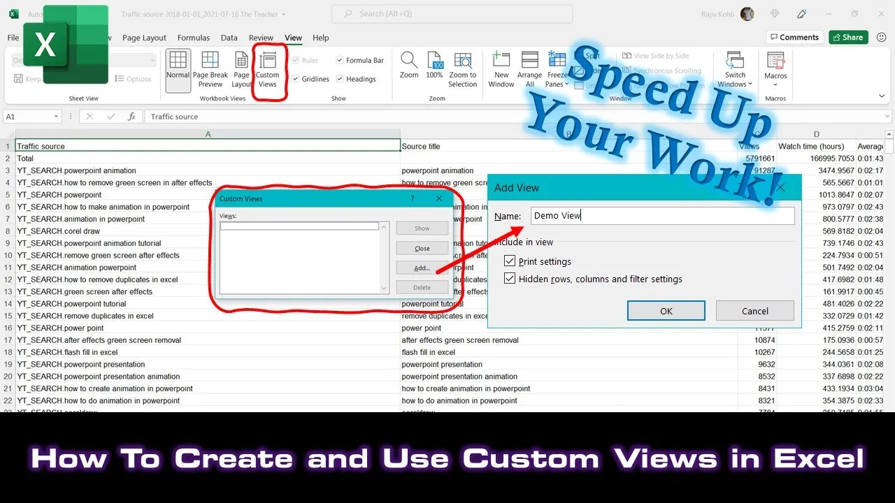
1. Click on the “View” tab from the Excel Ribbon.
2. Select “Custom Views” from the “Workbook Views” section.
3. Click “Add,” and give your Custom View a name, e.g., “Full View.” You can choose to include hidden rows, columns, and filter settings.

Now, whenever you need to switch between hiding and unhiding columns, you can easily select the appropriate Custom View, eliminating the need to perform this action manually each time.

Example 2: Applying Filters
Suppose you regularly work with specific filter settings, such as viewing only records for “British Columbia.” Create a Custom View for this filter configuration. Here’s how:

1. Apply the desired filter settings to your worksheet.
2. Go to the “View” tab, select “Custom Views,” and click “Add.”
3. Name this Custom View, e.g., “British Columbia.”

Now, switching to this Custom View will instantly apply the filter settings, saving you time and ensuring consistency in your data analysis.

Example 3: Page Layout Settings
For printing purposes, you may need to change page settings, such as page size, margins, and orientation. Create two Custom Views—one for display and one for printing. Here’s how to set them up:

1. Adjust the page settings according to your needs, e.g., one for viewing (“Display View”) and another for printing (“Printing View”).
2. In the “View” tab, choose “Custom Views” and click “Add” for each view.

Now, you can effortlessly switch between these Custom Views when you need to work on the worksheet or prepare it for printing.

Viewing Multiple Workbooks Side by Side
When working with multiple workbooks simultaneously, you can create a Custom View for this as well. This enables you to quickly set up and view your workbooks side by side. When the need arises, you can switch to this Custom View for added convenience.

Conclusion:
Custom Views in Microsoft Excel are a valuable tool for streamlining your work processes and saving time. You can create and manage multiple views with distinct display settings, ensuring that your worksheets are always ready for specific tasks. We hope you found this video informative and that Custom Views will enhance your Excel experience. Don’t forget to leave your comments, hit the thumbs-up button, and share this video with your friends. For more useful lessons, subscribe to our channel or visit our channel page. Thanks for watching, and take care!