
In today’s tutorial, we’ll delve into the world of Excel 2016, exploring the magic of custom lists and data validation. Whether you’re a seasoned Excel user or just starting, these techniques can significantly enhance your productivity. I’ve also prepared a detailed video tutorial for a visual walkthrough, and you can download the presentation file for hands-on practice.
Watch the tutorial video here
Understanding Custom Lists:
In Excel 2016, custom lists are a game-changer for efficiently populating repetitive data. To access the custom list option, navigate to the “File” menu, click on “Options,” select “Advanced,” and find the “Edit Custom List” button. In the dialog box, predefined lists like months or custom lists can be utilized to streamline data entry.
You can easily fill in sequences by dragging down from the initial value, and a neat trick involves double-clicking on the fill handle to generate a list up to the maximum used rows. Additionally, creating your own custom list is straightforward. Select the desired cells, go to “File,” “Options,” and then “Edit Custom List.” This can save time, especially when dealing with frequently used data.
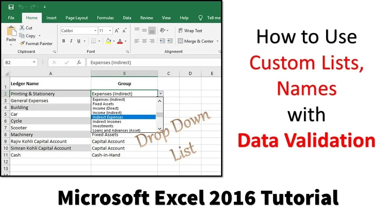
Data Validation for Streamlined Input:
Now, let’s explore how data validation coupled with custom lists can elevate your Excel game. In the “Groups” sheet, I’ve compiled a list of frequently used names. By selecting the entire column and naming it, we create a dynamic reference point. This list can then be used for data validation in other sheets.
Navigate to the desired column, go to “Data,” select “Data Validation,” choose “List,” and input the name you assigned earlier. This creates a convenient dropdown menu for quick and accurate data selection.
Enhancing Efficiency with Data Validation:
The real power lies in the ability to expand these lists dynamically. For instance, adding a new entry in the “Groups” sheet reflects instantly in the dropdown menu, ensuring that your lists are always up-to-date.
Application in Ledger Entries:
In the example, we extend this concept to ledger entries. By naming the entire column and applying data validation, we create dropdowns for easy selection. Even new entries, like adding a new account under a specific group, seamlessly integrate into the existing dropdown options.
Conclusion:
Mastering custom lists and data validation in Excel 2016 can significantly streamline your workflow, saving time and reducing the chance of errors. The dynamic nature of these features ensures that your lists evolve with your data. In the next tutorial, I’ll demonstrate how to leverage IF commands for more advanced data manipulation, leading to the creation of a comprehensive balance sheet.
I hope you found this tutorial insightful! If you have any questions or suggestions, drop a comment below. Don’t forget to like, share, and subscribe for more Excel tips and tricks. Stay tuned for the next tutorial, and have a productive day!